ECT 263 Week 5 Lab Assignment Help | Devry University 

Week 5 Lab Question 1

iLab5—Phase Locked Loop S-curve Using Tutor*Tims

(Filename convention: first initial last name PLLTT1 .doc)

Part A—Experiment Setup

Using Tutor*Tims, create the signal generator and phase locked loop circuit shown below.

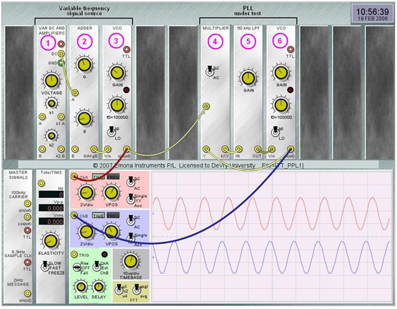
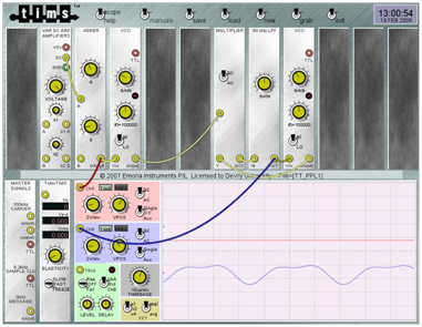
Figure 1

This circuit consists of two sections; the variable frequency signal source (modules 1–3) and the phase locked loop itself (modules 4–6).

 

You can use the positions of the knobs shown as a starting point. One setting that is particularly important is that the idle frequency of the signal source VCO and the PLL VCO must be the same. In this case, note that both are set for f0 = 100000. Both of the VCO’s idle frequencies are set to 100KHz.

 

The Voltage control on the Variable DC and Amplifiers module (module 1) controls the voltage to the signal source VCO and hence its frequency.

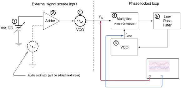
The figure below shows a block diagram of what we have created thus far.

Figure 2

The oscilloscope traces show that the PLL’s VCO is synchronized with the incoming signal source’s VCO.

 

What you need to do is to vary the input frequency (by varying the voltage produced by the Variable DC [module 1]) and seeing what effect that has on the PLL.

 

We want to create an S-curve characteristic of the PLL that shows the tracking range where the PLL’s VCO is locked onto the incoming signal. To do this, we will need to vary the input frequency and measure the error voltage as the PLL’s VCO adjusts to stay in sync with the incoming signal. We will need to use Tutor*Tims’ built-in metering to do this.

 

On the bottom half of Tutor*TIMS you will see a module just to the left of the scope titled simply Tutor TIMS. This module has an input that can be used to measure frequency and voltage. The module also has a control labeled Elasticity, which controls the droopiness of the wires and a switch that controls the speed of the signal processing. Set the speed switch to Fast.

 

In the process of taking our measurements, we will need to switch between the voltmeter function and the frequency counter function. Figure 3 below shows the alternating connections to take these measurements.

 

 

 

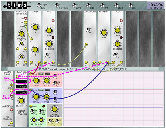
Figure 3

The dashed purple lines show the two alternate connections that we will be using to take our measurements. When you connect the metering unit to the VCO output (module 3), you will be measuring the input frequency applied to the PLL from the variable signal source. When you connect the metering unit to the 60KHz LPF (module 5) you will be measuring the resulting error voltage needed to keep the PLL’s VCO in sync with the incoming signal.

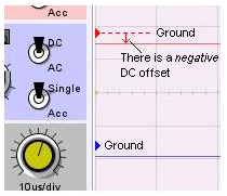
Initially in Figure 1 above, the scope was displaying the outputs of the two VCOs. Now, in Figure 3, it’s displaying the DC voltages applied to the VCOs. Figure 1 shows a more traditional view of a PLL where one can see whether the two signals are in phase or not. In this experiment, we need to measure the RMS value of the DC error voltage. If you’ll recall from your basic electronics, RMS is the DC equivalent of an AC signal. There is no such thing as a negative RMS voltage. So, to help us out we will use the scope, which can show a DC offset just fine, to tell us whether the number that we read on the RMS voltmeter is positive or negative. Look for two small triangles on the scope display (Figure 4). 

Part B—Recording Your Data

Now you are ready to record your data. Open an Excel spreadsheet. Label the left-hand column fIN. Label the right-hand column Error voltage. Start by connecting the metering input to the error voltage output of the low-pass filter (module 5). Wait for the voltage to stabilize. Record the voltage (paying attention to whether it’s above or below the ground reference on the scope. Move the metering input lead to the output of the PLL VCO (module 6) and record the frequency. (The graphic above the display may say Hz but in this case it is actually KHz.) 

Move the metering input back to the error voltage. Gradually change the input frequency by adjusting the DC voltage produced by the variable DC source (module1). Again, wait for the reading to stabilize and record it. Move the lead back to the input frequency (output of the first VCO [module 3]) and again record the frequency.

Construct a table of data in Excel. In all, you should have 5–10 data points within the tracking range and two to three above and two to three below the tracking range. fIN is your independent variable that you record in the left-hand column in Excel. Keep your data points in order. That is, make sure that your data goes from the lowest frequency to the highest frequency like what was done in the lecture section in eCollege. We want to see what happens to the error voltage as we vary the input frequency.

Figure 5 below shows what the error voltage will look like when you exceed the tracking range in either direction.

The blue trace is the error voltage output of the low-pass filter. You can see that it jumps around wildly as the PLL tries—unsuccessfully—to stay synchronized with the input signal.

 

Part C—Plotting Your Data

 

Once you’ve recorded enough data points in your Excel table, highlight the entire table (including the headings) and select the Chart Wizard. Then select x-y scatter plot and format the graph as you see fit. (Titles, background, etc., is your choice.) Make sure that all of your data is clearly understandable to the reader 

Use the Grab button to capture a sample of your circuit and paste it into the PLLTT1 answer sheet. It doesn’t matter which data point you grab—just a typical representative screen shot of your experiment in progress.

 

Copy your data table from Excel and paste it into the answer sheet.

 

Copy your completed graph from Excel and paste that into the answer sheet.

 

Submit your answer sheet document to the eCollege Dropbox.