For studying standard error first we
need to know what sampling distribution is:
Sampling distribution of a
statistic:
If we draw a sample of size ‘n’ from the given finite population of size N, the possible samples are NCn = k (say)
For each of these ‘K’ samples we can compute some statistic t= t(x1,x2….xn), in particular the mean and the the variance are given below.
Column
1 Column
2 Column
3 Column
4 Sample
Number Statistic t X S2 1 t1 X1 S12 2 t2 X2 S22 3 t3 X3
S32 : : : ; k tk Xk Sk2
The set of the values of the
statistics so obtained one for each sample constitutes ‘sampling distribution’
of the statistics.
For example the values t1,t2,...tn determine the sampling
distribution of the statistics ‘t’. In other words, statistics may be regarded
as a random variables which can take the values t1,t2...tn
and compute the various statistical constants for example mean ,variance,
skewness, kurtosis etc. for its distribution.
For example , the mean and variance of the sampling distribution of the
statistics ‘t’ is given by-
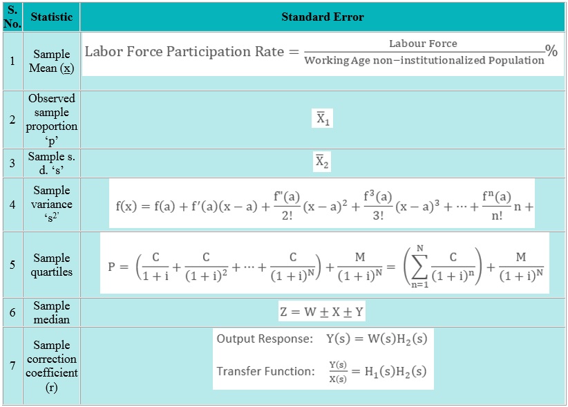
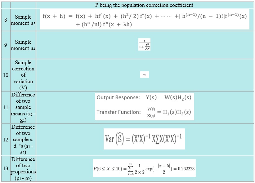
Definition of Standard Error The standard deviation of a
sampling distribution is known as its standard error , abbreviated as S.E.
Utility of Standard Error Standard error plays a very
important role in statistics. Standard error is important in large
sample theory and hypothesis testing.
Thus, if the discrepancy between the
observed and expected (hypothetical) value of statistic is greater than Z times
its S.E., the null hypothesis is rejected at level of significance. Hence, if | t - E(t)| Z *
S.E (t), The deviation is regarded insignificant
at 5% level of significance( is commonly take as 5%) .
The deviation is regarded
insignificant at 5% level of significance( is commonly take as 5%). The magnitude of the standard error
gives an index of the precision of the estimate of the parameter, the
reciprocal of the standard error is computed as the measure of reliability or
precision of the statistic. For Example, In Case of Proportion
In other words, the standard error
of ‘p’ and ‘’ vary inversely as the square root of the sample size. Thus, in
order to double the precision it amounts to reducing the standard error one half,
the sample size has to be increased 4 times.
Examples of on Standard Error
A die is thrown 9000 times in which
a throw of 3 or 4 is observed 3240 times. Show that Dad cannot be regarded as
an unbiased one and find the probable limits between which the probability of a
throw of 3 or 4 lies. If the coming of 3 or 4 is called a
success then in usual notations under the null The hypothesis, n=9000 X = number of successes Under the null hypothesis H0
that the die is an unbiased one we get, P= probability of success=
probability of getting a 3 or 4 = ⅙
+ ⅙ = ⅓ Alternate hypothesis will be die is
biased. H1: p 1/3
Since |Z| > 3 die is not
biased. Which provides evidence against Null hypothesis ,hence we reject null
hypothesis and accept alternate hypothesis. Finding the Limits between which the
probability of 3 or 4 lies: Since, die is not unbiased, P ⅓ A random sample of 500 pineapples
was taken from large consignment of 65 was found to be bad so that the standard
error of the population of bad ones in a sample of this size is 0.015 and
deduce that the percentage of bad pineapples in the consignment obtained
almost certainly lies between 8.5 and 17.5. Here we have, n= the sample size = 500 X = number of bad pineapples in the
sample = 65 P= Proportion of bad pineapples in
the sample = 65/ 500 = 0.13 since ‘P’ the proportion of bad
pineapples in the consignment is not known to us we may (take as in the last
example) an estimate of ‘P’ as p. Hence, p = 0.13, q= 0.87
Thus, the limits for the proportion
of bad pineapples in the consignment almost certainly lies between 8.5 and
17.5. Question:
A
random sample of 500 apples was taken from a large consignment and 60 were
found to be bad. Obtain the 98% confidence limits for the percentage of bad
apples in the consignment. Answer:
we have, P = proportion of bad apples in a
sample = 60 / 500 = 0.12 Since, significant value of Z
at 98%confidence limit coefficient( 2% level of significance) is 2.33(from
normal tables) => 98% confidence limits
for population proportions are :
Hence, 98% confidence limits are
(0.08615,0.15385).
We have, Z = (X - E(X))/ S.E.(X) = (X - nP)/ ~ N(0,1), since n is large
Now Z = (3240 - 9000 * 1/3)/
=> we take estimate of ‘P’ say ‘p’,
probability
of getting 3 or 4 almost lies between 0.345 and 0.375.


 USA
USA  India
India